Excel Integration Part 2: Build Advanced Marketo Reports and Data Visualizations Using Power Pivot and Power View

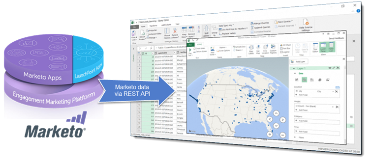
This is the second in a series of two articles that explain how to leverage the Power BI technology built into Microsoft Excel to create a true self-service business analytics experience with Marketo.

With the concepts covered in these articles, you’ll be able to:

• Import data from Marketo into Excel
• Import and combine data from other sources (SaaS applications, databases, flat files, etc.)
• Shape data for business needs and analysis purposes
• Refresh data on demand within Excel
• Create calculated columns and measures using formulas
• Create relationships between heterogeneous data
• Analyze data and build advanced reports with Pivot Tables and Pivot Charts
• Produce stunning data visualizations

Power Pivot and Power View for Excel

In this article, we provide examples of how to build the following:

• Advanced Marketo reports that leverage relationships between different collections of Marketo data using Power Pivot
• Cool static and animated visualizations using Power View

Power Pivot is an Excel add-in, already included in Excel 2016, you can use to perform powerful data analysis and create sophisticated data models. With Power Pivot, you can mash up large volumes of data from various sources, perform information analysis rapidly, and share insights easily. Data extracted from different data sources with Power Query can be sent to the data model, to the Excel spreadsheet, or to both. In the first article, we imported and shaped data from Marketo and sent it to the data model in order to perform more sophisticated analysis prior to making it available on the spreadsheet.

Power View is an alternative to the Excel visualization layer. It is an interactive data exploration, visualization, and presentation experience that encourages intuitive ad-hoc reporting and dashboarding.

The Marketo Power Workbook

Download Workbook

In the first article, we covered the data import and shaping process using Power Query technology. We learned how to implement some advanced power queries in order to extract leads and activities from Marketo. Because some of you would want to jump directly to the point where they build reports and visualisations, without coding, we released the Marketo Power Workbook that you can download here.

This workbook contains all the queries detailed in the first article and a few more. We improved the error handling and added some extra parameters in the configuration worksheet. If you went through the first article, we still recommend you to download the Marketo Power Workbook and check out what has been added.

Configure Workbook

Please check out the Prerequisites and the Power Query Workbook Creation sections from the first article in order to understand the prerequisites and how to configure the Marketo configuration worksheet.

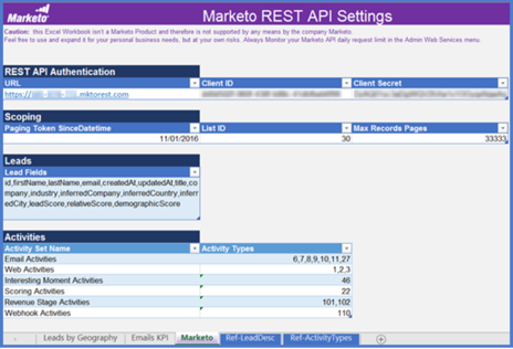
Fill in all of the required information from the Marketo configuration worksheet:

• Marketo REST API Authentication: required
• Scoping: set the Paging Token SinceDatetime and the Id of your Marketo static list containing all the leads you want to analyze
• Leads: for the reports to come, you must at least specify the following Lead fields: id, firstName, lastName, email, createdAt, updatedAt, title, company, industry, inferredCountry, inferredCity
  • If the city information is more accurate in one of your custom fields, then you can use your own field instead
• Activities: Activity types to fetch from the Marketo database are specified here for each Activity set, no need to change this now.
  • Note that we provided a utility query on the workbook that lists, right on the Excel workbook, all the existing Activity types if you want to adjust this information later on

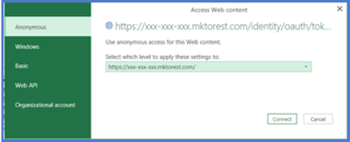
Note that you may see some security related pop-ups. Trust external connections and set them to ‘Public’.

If you see the pop-up below, stay with ‘Anonymous’ web access content. The authentication to Marketo is directly managed by our custom queries, so no need to enable any other kind of access.

Download Marketo Data

Make sure first that the parameter you define in the Scoping area of the Marketo configuration worksheet will not result in downloading too much data, exceeding your Marketo API daily request limit (see first article).

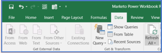
When ready, click the ‘Refresh All’ button from the ‘Data’ menu and wait that all the data is downloaded into the workbook.

If formatting error messages are displayed when downloading the data, similar to ‘column1 not found’, that means one or more queries are failing to get the data, so the formatting is also failing. Try again later on, if the error persists, then check your version of Excel (do not use Excel 2016 from Office 365).

It is important also to respect the latency from the Marketo platform. If you do any changes in a static list, or in your lead data, then it is preferable to wait before launching the Power Queries.

Data Modeling in Power Pivot

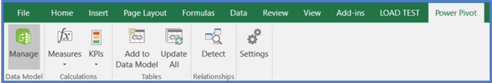
Open Power Pivot by clicking the ‘Manage’ button from the Power Pivot menu, available in the top menu bar (if not available check your version of Excel, Power Pivot can be installed as an add-in in some versions of Excel).

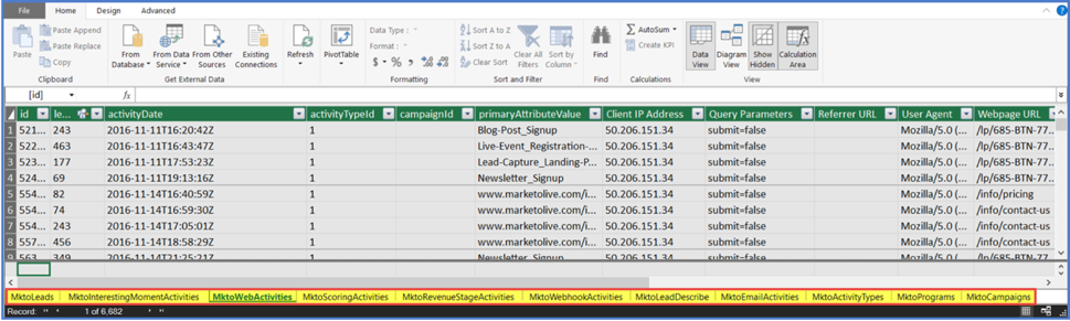
All the data downloaded from Marketo and sent to the data model should be accessible from the different tabs at the bottom of the Power Pivot window.

Data Analysis Expressions (DAX)

We need to enrich or reformat the data for some reports. Let’s use Power Pivot Data Analysis Expressions (DAX) to define some custom calculations as calculated columns and measures (also known as calculated fields). See the ‘DAX in Power Pivot’ link in the References section to learn more about DAX.

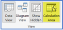
Make sure the Calculation Area is showing in the Power Pivot window; if not, enable it from the Power Pivot Home menu.

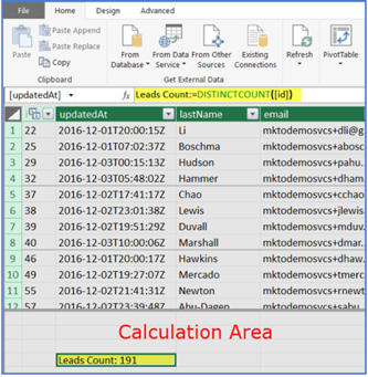
Select the MktoLeads tab and add the Leads Count measure anywhere in the Leads Calculation Area: Leads Count:=DISTINCTCOUNT([id]).

This measure is counting the distinct leads available in the list, based on their id. It would also take into account the eventual filters in place in the context of a report.

This measure is not really necessary since the reports are capable of summing up the number of leads but we did it in order to have a lead count with a nicer name than ‘sum of MktoLeads’. It is also a simple example that let you easily imagine some more complex measures doing averages, min, max for a specific type of data entry (e.g. all the leads with a score higher than 50, average score, etc …).

Now let’s select the MktoWebActivities tab and create three calculated columns.

Insert the following calculated columns by scrolling to the far right of the table and by clicking the column ‘Add Column’.

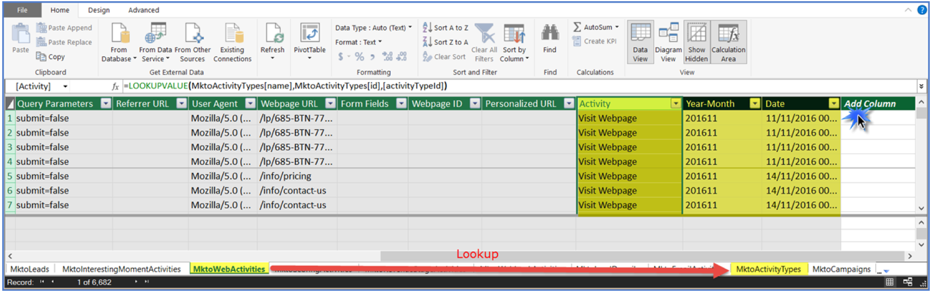
Activity: Obtain the user-friendly Activity label by looking up the Activity Id in the table MktoActivtyTypes.

=LOOKUPVALUE(MktoActivityTypes[name],MktoActivityTypes[id],[activityTypeId])

Year-Month: reformat the Activity date with a pattern ‘YYYYmm’ that is more suitable for some reports.

=LEFT([activityDate],4)&MID([activityDate],6,2)

Date: Activity Date is just a String from our original query, transform it to a proper date.

=DATE(LEFT([activityDate],4),MID([activityDate],6,2),MID([activityDate],9,2))

Now let’s create the three same measures for the MktoEmailActivities tab, and 2 additional ones:

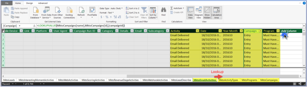
Campaign: Obtain the user-friendly Campaign name by looking up the Campaign Id in the table MktoCampaigns.

=LOOKUPVALUE(MktoCampaigns[name],MktoCampaigns[id],[campaignId])

Program: Obtain the user-friendly Program name by looking up the Campaign Id in the table MktoCampaigns. The table MktoPrograms can provide more details about the Program such as folder, workspace, etc.

=LOOKUPVALUE(MktoCampaigns[programName],MktoCampaigns[id],[campaignId])

Entity-Relationships

We saw previously a way to lookup information from another table within the model in order to complete some missing information. Power Pivot offers a more powerful option to define the relationships between some tables of the data model, allowing us to leverage those relationships directly from the reports. Let define the key relationships for our reports.

Select the Diagram View from the Power Pivot window.

Trace the following relationships within the Data model diagram:

• MktoInterestingMomentActivities:leadId → MktoLeads:id
• MktoScoringActivities:leadId → MktoLeads:id
• MktoRevenueStageActivities:leadId → MktoLeads:id
• MktoWebActivities:leadId → MktoLeads:id
• MktoEmailActivities:leadId → MktoLeads:id

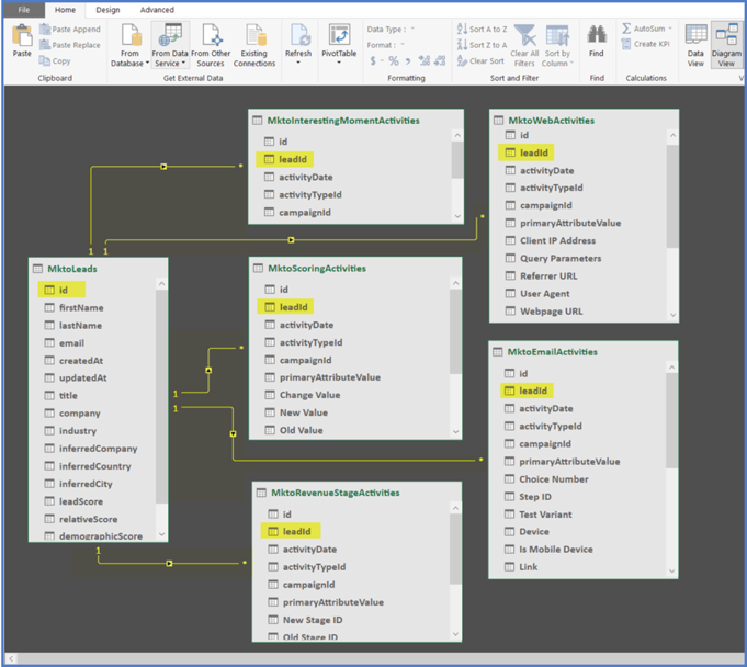
We’ll not use all of these relationships and objects in our reports, only the Leads, Web Activities and Email Activities.

Now it’s time to build some reports.

Emails Performance Pivot Chart

This first report is showing email performance KPIs based on a standard Excel Pivot Chart. It allows us to filter data by Industry and/or Campaign.

You can create a Pivot Chart right from the Power Pivot menu by selecting ‘Pivot Chart’ from the ‘Pivot Table’ selector.

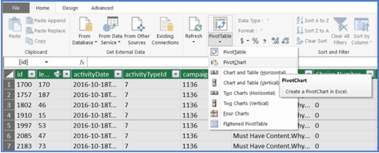
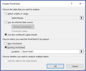
An alternative is to create a Pivot Chart directly from the Excel spreadsheet, ticking the option ‘Use this workbook’s Data Model’.

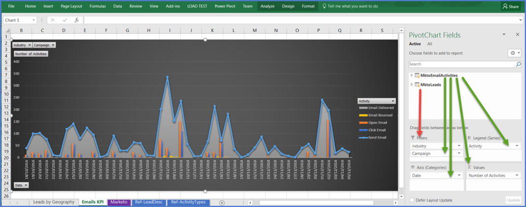
Drag and drop the fields from the MktoEmailActivities and the MktoLeads tables, like the figure below:

MktoEmailActivities.Activity → Legend (this use the DAX calculated column we implemented on MktoEmailActivities earlier)

MktoEmailActivities.Date → Axis (this use the DAX calculated column we implemented on MktoEmailActivities earlier)

MktoEmailActivities.Id → ∑ Values

MktoEmailActivities.Campaign → Filter

MktoLeads.industry → Filter

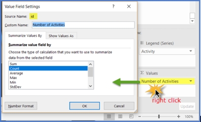
You can create custom name by selecting ‘Value Field Settings’ on each dropped field. In this case, we dropped the Email Activity id field into the ‘∑ Values’ section and edited its custom name as ‘Number of Activities’.

Now let’s configure the Pivot Chart. Right click directly on the chart and select the ‘Change Chart Type’ option in the contextual menu.

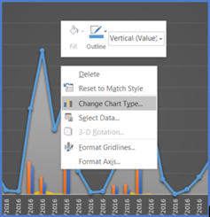
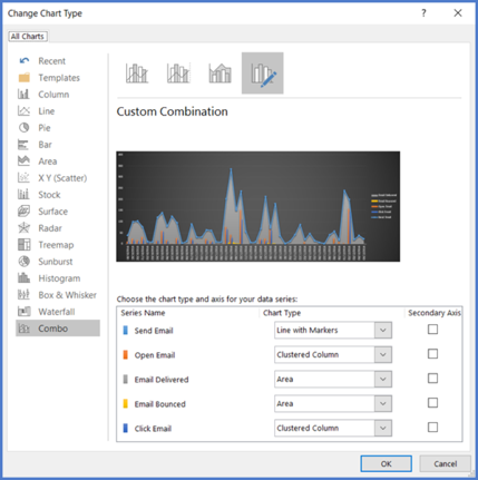
And this is how we selected the different chart type for all data series.

Leads Map with Power View

The second report displays your Leads and Contacts by geography on a world map and by Industry.

We’ll need Power View for this report. Please follow the reference link below ‘Turn-on Power View in Excel 2016’ in order to turn on the menu in Excel. Or you can just type ‘power view’ in the Excel search box.

Select ‘Insert a Power View Report’.

On the blank Power View report, select the MktoLeads table on the right panel and drag & drop the lead location field (e.g. inferredCity). Now the menu ‘Design’ appear in the main menu.

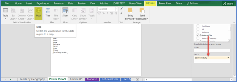
Switch to the Map visualization by selecting ‘Map’ in the Power View ‘Design’ menu.

Drag and drop the fields from the MktoLeads table, like the figure below:

MktoLeads.industry → Color

MktoLeads.inferredCity → Locations

MktoLeads.Leads Count → ∑ Size (this use the DAX measure we implemented on MktoLeads earlier)

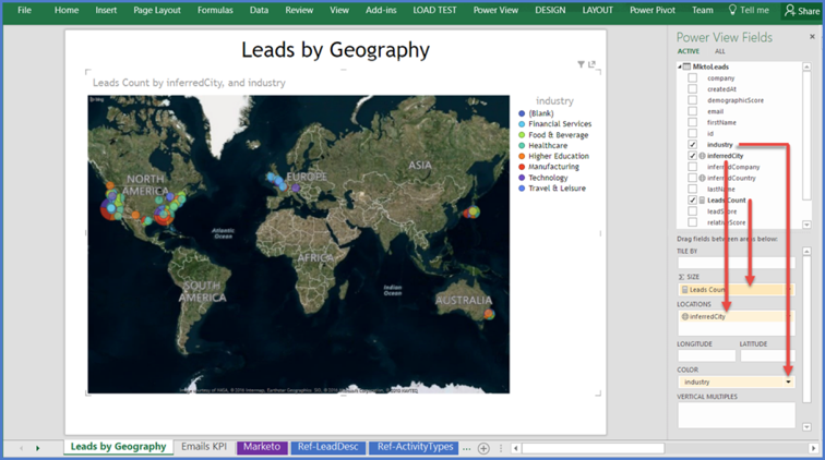
And your Leads map is ready! You just need to adjust the size of the map, customize the title and legends.

Power View allows you to build advanced dashboards with multiple graphs on one single spreadsheet. Check out the referenced tutorial below ‘Create Amazing Power View Reports’ to see how to proceed with more dashboard components with Power View.

Web Activities Animated on a 3D Map

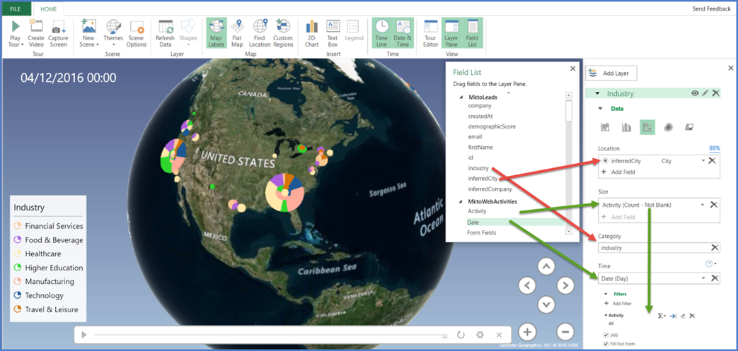
This third report displays your Lead web activities, by industry, on a 3D world map.

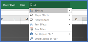
We’ll need a 3D Map for this report. Just type ‘3D’ in the Excel search box and select ‘3D Map’.

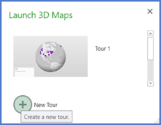
Create a new tour from the pop-up window.

Select the Bubble Chart on the right panel.

Drag and drop the fields, from the MktoLeads and the MktoWebActivities tables, like the figure below:

MktoLeads.industry → Category

MktoLeads.inferredCity → Location

MktoWebActivities.Activity → Time (this use the DAX calculated column we implemented on MktoWebActivities earlier. The id field could also be used for counting activities.)

MktoWebActivities.Date → Time (this use the DAX calculated column we implemented on MktoWebActivities earlier)

MktoWebActivities.Activity can also be used as a filter to filter out the different types of web activities.

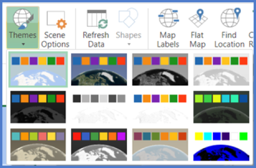
Use the ‘Themes’ button in order to change the color scheme of your 3D Map.

Open the ‘Scene Options’ in order to customize your animations.

And you’re done with the 3D World Map, now you can have fun animating the globe and creating video from it. 

Next Steps

We just scratched the surface of what is possible to do with the Excel Power BI tools. We recommend you to search the web for other great articles and tutorials to expand your Excel skills and design the reports you need to achieve your business goals.

We hope you enjoyed these articles and that they helped you leverage the great benefits of Excel and Marketo combined.

References

Power Pivot

• Power Pivot: Powerful data analysis and data modeling in Excel
• Data Analysis Expressions (DAX) in Power Pivot

Power View

• Turn-on Power View in Excel 2016
• Tutorial: Create Amazing Power View Reports